Multi-task Loss
This is a short review of the paper titled "Multi-Task Learning Using Uncertainty to Weigh Losses for Scene Geometry and Semantics" by Kendall et al, 2018 .

This is a short review of the paper titled "Multi-Task Learning Using Uncertainty to Weigh Losses for Scene Geometry and Semantics" by Kendall et al, 2018 .
Problem description
Given a model with multiple heads(tasks), how to balance all the losses ? The gradients are affected by the magnitude of losses, and naturally the tasks with higher loss magnitudes are prioritized.
Key Contribution
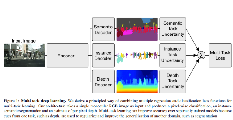
The author uses the example of a multi-head model predicting semantic segmentation, instance segmentation and inverse depth in this paper to demonstrate his experiment.
Core idea
-
Let each model branch predict its own homoscedastic uncertainty
-
Weigh each loss by the branch's respective uncertainty
Proof
Let \( f^W(x) \) be the output of a neural network with weights \( W \) on input \( x \). For regression tasks we define our likelihood as a Gaussian with mean given by the model output :
Multi task likelihoods can be defined as (assuming independent random variables) :
The probability density of observing a single data point x, that is generated from a Gaussian distribution is given by:
Substituting \ref{3} in \ref{1}, Log likelihood for multi task input can be defined as:
Now let's assume that our model output is composed of two vectors y1 and y2, each following a Gaussian distribution such that:
Taking log on both sides and expanding \ref{5} using \ref{4}, we get:
As \( \sigma_{1} \) (the noise parameter for the variable \( y_{1} \) ) increases, weight of \( \mathcal{L}_{1} \) decreases. On the other hand, as the noise decreases, the weight of the respective objective increases. The noise is discouraged from increasing too much (effectively ignoring the data) by the last term in the objective, which acts as a regulariser for the noise terms.
In practice, we train the network to predict the \( \sigma^{2} \). This is numerically more stable than regressing the variance, \( \sigma \), as the loss avoids any division by zero.
Results
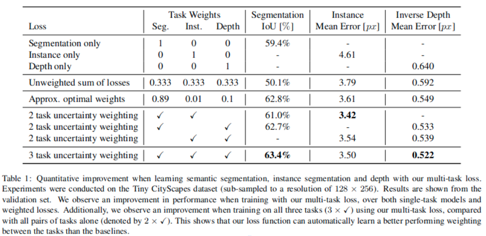
A reasonably well trained model is obtained without the need for manual loss weight adjustment. There's a minor improvement observed in segmentation + inverse depth metrics.